library(gxc)
library(sf)
library(dplyr)
library(purrr)
library(ggplot2)
library(stringr)
library(tidyr)
library(plotly)
library(rnaturalearth)
library(bench)
library(future)Performance
Packages used in this section
How long will linking take on an average laptop?
Depending on the size and extent of your data, running gxc linking functions can take a very long time. After all, we are dealing with continuous data on a national to global level! Generally, there are two steps that take up the majority of the time: 1. Data downloads and 2. raster extraction. In this section, we diagnose performance and we also explore options with the potential to improve performance.
When thinking about performance in spatio-temporal applications, there are four key characteristics of a dataset that affect the computational complexity:
- Sample size: 10 or 100,000 people?
- Spatial extent: City, national, continental, or worldwide?
- Observation period: Averages for month, season, or year?
- Baseline period: No baseline, 10y baseline, or 30y baseline?
To exemplify, we will create an example grid with varying sample sizes (10 to 5,000) and observation periods (0 days, 2 days, 11 days). You can expand the collapsed code below to see how we created the data.
Code to create example data
# Retrieve geometries
germany <- ne_countries(
  country = "Germany",
  scale = "medium",
  returnclass = "sf"
)

europe <- ne_countries(
  continent = "Europe",
  scale = "medium",
  returnclass = "sf"
) |>
  st_intersection(st_as_sfc(st_bbox(c(
    xmin = -10.0,
    ymin = 35.0,
    xmax = 40.0,
    ymax = 71.0
  ), crs = st_crs(4326))))

# Generate grids
grid_ger <- st_bbox(germany) |>
  st_as_sfc() |>
  st_make_grid(n = c(100, 100)) |>
  st_sf(geometry = _)

grid_eu <- st_bbox(europe) |>
  st_as_sfc() |>
  st_make_grid(n = c(100, 100)) |>
  st_sf(geometry = _)

get_corners <- function(grid) {
  bbox <- st_bbox(grid)
  corners <- st_sfc(
    st_point(bbox[c("xmin", "ymin")]),
    st_point(bbox[c("xmax", "ymin")]),
    st_point(bbox[c("xmin", "ymax")]),
    st_point(bbox[c("xmax", "ymax")]),
    crs = st_crs(grid)
  )
  corners <- st_within(corners, grid)
  attributes(corners) <- NULL
  names(corners) <- c("ll", "lr", "ul", "ur")
  unlist(corners)
}

# Sample-function (always including the four corner cells).
sample_grid <- function(n, grid, seed = NULL) {
  if (n < 4) stop("n must be at least 4 to include all corner cells.")

  # Calculate n-corner polygons
  corners <- get_corners(grid)
  n_random <- n - length(corners)

  # Exclude the corner cells from the random sample
  remaining <- grid[-corners, ]

  # Randomly sample from the remaining cells
  set.seed(seed)
  random_sample <- remaining[sample(nrow(remaining), n_random), ]

  # Combine the corner cells with the random sample
  rbind(grid[corners, ], random_sample)
}

# Sample grids with various n
sample_sizes <- c(10, 20, 50, 100, 200, 500, 1000, 2000, 5000)

# Loop over the sample sizes
samples_ger <- lapply(sample_sizes, sample_grid, grid_ger)
samples_eu <- lapply(sample_sizes, sample_grid, grid_eu, seed = 111)
samples <- c(samples_ger, samples_eu)
names(samples) <- sprintf("%s_sample_%s", rep(c("ger", "eu"), each = length(sample_sizes)), sample_sizes)
The data consists of 18 lists containing vector cells with a varying sample size:
str(samples, max.level = 1, give.attr = FALSE)List of 18
$ ger_sample_10 :Classes 'sf' and 'data.frame': 10 obs. of 1 variable:
$ ger_sample_20 :Classes 'sf' and 'data.frame': 20 obs. of 1 variable:
$ ger_sample_50 :Classes 'sf' and 'data.frame': 50 obs. of 1 variable:
$ ger_sample_100 :Classes 'sf' and 'data.frame': 100 obs. of 1 variable:
$ ger_sample_200 :Classes 'sf' and 'data.frame': 200 obs. of 1 variable:
$ ger_sample_500 :Classes 'sf' and 'data.frame': 500 obs. of 1 variable:
$ ger_sample_1000:Classes 'sf' and 'data.frame': 1000 obs. of 1 variable:
$ ger_sample_2000:Classes 'sf' and 'data.frame': 2000 obs. of 1 variable:
$ ger_sample_5000:Classes 'sf' and 'data.frame': 5000 obs. of 1 variable:
$ eu_sample_10 :Classes 'sf' and 'data.frame': 10 obs. of 1 variable:
$ eu_sample_20 :Classes 'sf' and 'data.frame': 20 obs. of 1 variable:
$ eu_sample_50 :Classes 'sf' and 'data.frame': 50 obs. of 1 variable:
$ eu_sample_100 :Classes 'sf' and 'data.frame': 100 obs. of 1 variable:
$ eu_sample_200 :Classes 'sf' and 'data.frame': 200 obs. of 1 variable:
$ eu_sample_500 :Classes 'sf' and 'data.frame': 500 obs. of 1 variable:
$ eu_sample_1000 :Classes 'sf' and 'data.frame': 1000 obs. of 1 variable:
$ eu_sample_2000 :Classes 'sf' and 'data.frame': 2000 obs. of 1 variable:
$ eu_sample_5000 :Classes 'sf' and 'data.frame': 5000 obs. of 1 variable:plot_samples <- bind_rows(samples[startsWith(names(samples), "ger")], .id = "sample")
ggplot(plot_samples) +
geom_sf(fill = "#c994c7", color = "#dd1c77", size = 0.3) +
geom_sf(data = germany, fill = NA, color = "#2c7fb8", size = 0.8) +
facet_wrap(~sample, ncol = 3, dir = "v", labeller = function(value) {
as.data.frame(paste("Sample =", gsub("ger_sample_", "", value$sample)))
}) +
theme_void()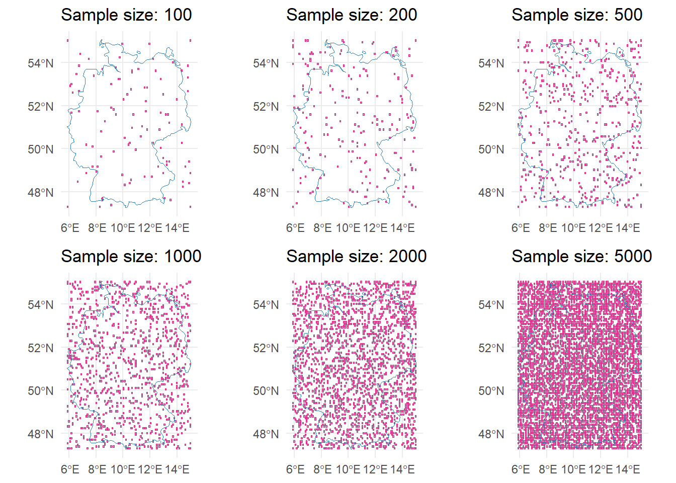
To analyse performance, we will run the following R code repeatedly. The curly braces indicate the function arguments that vary between function calls. Each of these calls is benchmarked 10 times to ensure the consistency of timings.
link_monthly(
  .data = {data with varying sample sizes},
  indicator = "2m_temperature",
  time_span = {varying time spans}
)
We use the 2m_temperature indicator from the ERA5-Land monthly averages for this exercise. The code was run on an average office laptop (Intel Core i7-10510U CPU, 16GB RAM, Windows 10). The benchmarking is powered by the bench package.
# Add arbitrary time identifier to grid
samples <- lapply(samples, function(grid) {
  grid$date <- "2020-12-01"
  grid
})

# Pre-cache (to keep timings consistent)
invisible({
  link_monthly(samples[[1]], indicator = "2m_temperature", time_span = 0)
  link_monthly(samples[[1]], indicator = "2m_temperature", time_span = 2)
  link_monthly(samples[[1]], indicator = "2m_temperature", time_span = 11)
  link_monthly(samples[[10]], indicator = "2m_temperature", time_span = 0)
  link_monthly(samples[[10]], indicator = "2m_temperature", time_span = 2)
  link_monthly(samples[[10]], indicator = "2m_temperature", time_span = 11)
})

time_spans <- c(0, 2, 11)

# Benchmark
bm <- bench::press(
  extent = c("ger", "eu"),
  sample_size = sample_sizes,
  time_span = time_spans,
  bench::mark(
    link_monthly(
      .data = samples[[sprintf("%s_sample_%s", extent, sample_size)]],
      indicator = "2m_temperature",
      time_span = time_span,
      verbose = FALSE
    ),
    iterations = 10
  )
)
# A tibble: 54 × 8
extent sample_size time_span min median `itr/sec` mem_alloc `gc/sec`
<chr> <dbl> <dbl> <bch:tm> <bch:tm> <dbl> <bch:byt> <dbl>
1 ger 10 0 180.05ms 190.62ms 5.25 886.66KB 0.583
2 eu 10 0 243.7ms 249.44ms 3.98 1.02MB 0.442
3 ger 20 0 273.27ms 281.14ms 3.51 1.95MB 0.390
4 eu 20 0 386.68ms 395.6ms 2.52 2.07MB 0.281
5 ger 50 0 546.53ms 552.62ms 1.80 4.9MB 0.450
6 eu 50 0 829.46ms 838.57ms 1.19 5.42MB 0.132
7 ger 100 0 998.2ms 1.02s 0.978 9.69MB 0.419
8 eu 100 0 1.61s 1.62s 0.618 10.87MB 0.412
9 ger 200 0 1.93s 1.96s 0.512 19.38MB 0.341
10 eu 200 0 3.06s 3.08s 0.324 20.93MB 0.216
# ℹ 44 more rowsCode for the interactive plot
bm$time_span <- sapply(
  as.character(bm$time_span),
  switch,
  `0` = "monthly",
  `2` = "seasonal",
  `11` = "yearly"
)

plots <- lapply(c("ger", "eu"), function(extent) {
  data <- bm |>
    filter(extent %in% !!extent) |>
    select(sample_size, median, time_span, time) |>
    mutate(
      min = sapply(time, min),
      max = sapply(time, max)
    ) |>
    unnest_longer(time)

  p <- ggplot(data, aes(x = sample_size, color = time_span, group = time_span)) +
    geom_point(aes(y = unclass(time))) +
    geom_line(aes(y = unclass(median))) +
    geom_ribbon(aes(ymin = min, ymax = max), alpha = 0.2, color = NA) +
    labs(
        title = "Execution time vs. sample size",
        x = "Sample size",
        y = "Execution time (in s)",
        color = "Observation period"
    ) +
    scale_color_manual(values = c(
        "month" = "#dd1c77",
        "seasonal" = "#225ea8",
        "yearly" = "#7fcdbb"
    )) +
    theme_minimal()

  ggplotly(p) |>
    style(p, visible = identical(extent, "ger"))
}) |>
  setNames(c("ger", "eu"))

vis_eu <- c(rep(FALSE, 7), rep(TRUE, 7))
vis_ger <- c(rep(TRUE, 7), rep(FALSE, 7))

menus <- list(
  list(
    type = "dropdown",
    active = 0,
    x = 0,
    y = 1.12,
    xanchor = "left",
    yanchor = "top",
    buttons = list(
      list(label = "Germany", method = "restyle", args = list("visible", vis_ger)),
      list(label = "Europe", method = "restyle", args = list("visible", vis_eu))
    )
  )
)

annot <- list(
  x = 0,
  y = 1.22,
  xref = "paper", yref = "paper",
  text = "Spatial extent",
  showarrow = FALSE,
  font = list(size = 14)
)

p <- plotly_build(plots$ger)
p$x$data <- c(plots$ger$x$data, plots$eu$x$data)
p <- p |>
  layout(updatemenus = menus, annotations = annot, margin = list(t = 150)) |>
  style(hovertemplate = "<i>Time</i>: %{y} s") |>
  config(displaylogo = FALSE, modeBarButtonsToRemove = c(
    "zoomIn2d", "zoomOut2d", "toImage", "hoverCompareCartesian",
    "hoverClosestCartesian", "resetScale2d", "autoScale2d", "lasso2d",
    "select2d", "pan2d", "zoom2d"
  ))
bm_parallel <- bench::press(
extent = c("ger", "eu"),
sample_size = sample_sizes,
time_span = time_spans,
chunk_size = c(50, 100, 200),
workers = c(2, 6),
bench::mark(
{
future::plan(future::multisession, workers = workers)
link_monthly(
.data = samples[[sprintf("%s_sample_%s", extent, sample_size)]],
indicator = "2m_temperature",
time_span = time_span,
verbose = FALSE,
parallel = TRUE,
chunk_size = chunk_size
)
},
iterations = 10
)
)# A tibble: 324 × 10
extent sample_size time_span chunk_size workers min median `itr/sec`
<chr> <dbl> <dbl> <dbl> <dbl> <bch:tm> <bch:tm> <dbl>
1 ger 10 0 50 2 439.5ms 445.12ms 2.24
2 eu 10 0 50 2 504.3ms 507.87ms 1.96
3 ger 20 0 50 2 646.51ms 657.86ms 1.51
4 eu 20 0 50 2 701.86ms 714.56ms 1.40
5 ger 50 0 50 2 1s 1.02s 0.985
6 eu 50 0 50 2 1.23s 1.25s 0.800
7 ger 100 0 50 2 1.56s 1.58s 0.632
8 eu 100 0 50 2 2.03s 2.09s 0.480
9 ger 200 0 50 2 2.56s 2.62s 0.382
10 eu 200 0 50 2 3.58s 3.62s 0.276
# ℹ 314 more rows
# ℹ 2 more variables: mem_alloc <bch:byt>, `gc/sec` <dbl>Code for the interactive plot
bm_parallel$time_span <- sapply(
  as.character(bm_parallel$time_span),
  switch,
  `0` = "monthly",
  `2` = "seasonal",
  `11` = "yearly"
)


part_plot <- function(ext, time, cs, workers) {
  data <- bm |>
    filter(extent %in% !!ext) |>
    filter(time_span %in% !!time) |>
    select(sample_size, median, time_span, time) |>
    mutate(
      min = sapply(time, min),
      max = sapply(time, max)
    ) |>
    unnest_longer(time)

  data_parallel <- bm_parallel |>
    filter(extent %in% !!ext) |>
    filter(time_span %in% !!time) |>
    filter(chunk_size %in% !!cs) |>
    filter(workers %in% !!workers) |>
    select(sample_size, median, time_span, time, chunk_size, workers) |>
    mutate(
      min = sapply(time, min),
      max = sapply(time, max)
    ) |>
    unnest_longer(time) |>
    mutate(
      chunk_size = factor(as.character(chunk_size), levels = c("50", "100", "200")),
      workers = factor(as.character(workers), levels = c("2", "6"))
    )
  data <- bind_rows("Sequential" = data, "Parallel" = data_parallel, .id = "execution")

  p <- ggplot(data, aes(x = sample_size, color = execution, group = execution)) +
    geom_point(aes(y = unclass(time))) +
    geom_line(aes(y = unclass(median))) +
    geom_ribbon(aes(ymin = min, ymax = max), alpha = 0.2, color = NA) +
    labs(
      title = "Execution time vs. sample size",
      x = "Sample size",
      y = "Execution time (in s)",
      color = NULL
    ) +
    scale_y_continuous(limits = c(0, max(unclass(bm$median)))) +
    scale_color_discrete() +
    theme_minimal()

    ggplotly(p) |>
      style(
        p,
        visible = identical(ext, "ger") &&
          identical(time, "monthly") &&
          identical(cs, 50) &&
          identical(workers, 2)
      )
}


plots <- lapply(c("ger", "eu"), function(ext) {
  lapply(c("monthly", "seasonal", "yearly"), function(time) {
    lapply(c(50, 100, 200), function(cs) {
      lapply(c(2, 6), function(workers) {
        part_plot(ext, time, cs, workers)
      }) |>
        setNames(c(2, 6))
    }) |>
      setNames(c(50, 100, 200))
  }) |>
    setNames(c("monthly", "seasonal", "yearly"))
}) |>
  setNames(c("ger", "eu")) |>
  list_flatten() |>
  list_flatten() |>
  list_flatten()


vis_ger <- grepl("ger", names(plots))
vis_monthly <- grepl("monthly", names(plots))
vis_seasonal <- grepl("seasonal", names(plots))
vis_yearly <- !vis_monthly & !vis_seasonal
vis_cs50 <- grepl("50", names(plots))
vis_cs100 <- grepl("100", names(plots))
vis_cs200 <- !vis_cs50 & !vis_cs100
vis_2workers <- grepl("2$", names(plots))
vis_6workers <- grepl("6$", names(plots))

menus <- list(
  list(
    id = "ext", type = "dropdown", active = 0, x = 0.175, y = 1.12,
    buttons = list(
      list(label = "Germany", method = "restyle", args = list("customdata", 0)),
      list(label = "Europe", method = "restyle", args = list("customdata", 1))
    )
  ),
  list(
    id = "time", type = "dropdown", active = 0, x = 0.425, y = 1.12,
    buttons = list(
      list(label = "Monthly", method = "restyle", args = list("customdata", 0)),
      list(label = "Seasonal", method = "restyle", args = list("customdata", 1)),
      list(label = "Yearly", method = "restyle", args = list("customdata", 2))
    )
  ),
  list(
    id = "cs", type = "dropdown", active = 0, x = 0.675, y = 1.12,
    buttons = list(
      list(label = "50", method = "restyle", args = list("customdata", 0)),
      list(label = "100", method = "restyle", args = list("customdata", 1)),
      list(label = "200", method = "restyle", args = list("customdata", 2))
    )
  ),
  list(
    id = "workers", type = "dropdown", active = 0, x = 0.925, y = 1.12,
    buttons = list(
      list(label = "2 workers", method = "restyle", args = list("customdata", 0)),
      list(label = "6 workers", method = "restyle", args = list("customdata", 1))
    )
  )
)

annot <- list(
  list(
    x = 0,
    y = 1.22,
    xref = "paper", yref = "paper",
    text = "Spatial extent",
    showarrow = FALSE,
    font = list(size = 14)
  ),
  list(
    x = 0.25,
    y = 1.22,
    xref = "paper", yref = "paper",
    text = "Observation period",
    showarrow = FALSE,
    font = list(size = 14)
  ),
  list(
    x = 0.63,
    y = 1.22,
    xref = "paper", yref = "paper",
    text = "Chunk size",
    showarrow = FALSE,
    font = list(size = 14)
  ),
  list(
    x = 0.965,
    y = 1.22,
    xref = "paper", yref = "paper",
    text = "Number of workers",
    showarrow = FALSE,
    font = list(size = 14)
  )
)

p <- plotly_build(plots$ger_monthly_50_2)
p$x$data <- lapply(plots, \(p) p$x$data) |> list_flatten()
p <- p |>
  layout(updatemenus = menus, annotations = annot, margin = list(t = 150)) |>
  style(hovertemplate = "<i>Time</i>: %{y} s") |>
  config(displaylogo = FALSE, modeBarButtonsToRemove = c(
    "zoomIn2d", "zoomOut2d", "toImage", "hoverCompareCartesian",
    "hoverClosestCartesian", "resetScale2d", "autoScale2d", "lasso2d",
    "select2d", "pan2d", "zoom2d"
  )) |>
    htmlwidgets::onRender("
    function(el, x) {
        var isUpdating = false;

        el.on('plotly_restyle', function(data) {
            // prevent infinite loops
            if (isUpdating) return;
            isUpdating = true;

            // get indices of all menus
            var m = el.layout.updatemenus;
            var ext_i = m[0].active || 0;
            var time_i = m[1].active || 0;
            var cs_i = m[2].active || 0;
            var work_i = m[3].active || 0;

            // calculate which traces should be visible
            // traces per combination = 3 * 2 (Seq & Par) = 6.
            var combo = (ext_i * 18) + (time_i * 6) + (cs_i * 2) + work_i;
            var tracesPerCombo = el.data.length / 36;
            var start = combo * tracesPerCombo;
            var end = start + tracesPerCombo;

            // create visibility array
            var vis = [];
            for (var i = 0; i < el.data.length; i++) {
                vis[i] = (i >= start && i < end);
            }

            Plotly.restyle(el, {visible: vis}).then(function() {
                isUpdating = false;
            });
        });
    }
  ")
How does gxc work?
Parallel processing
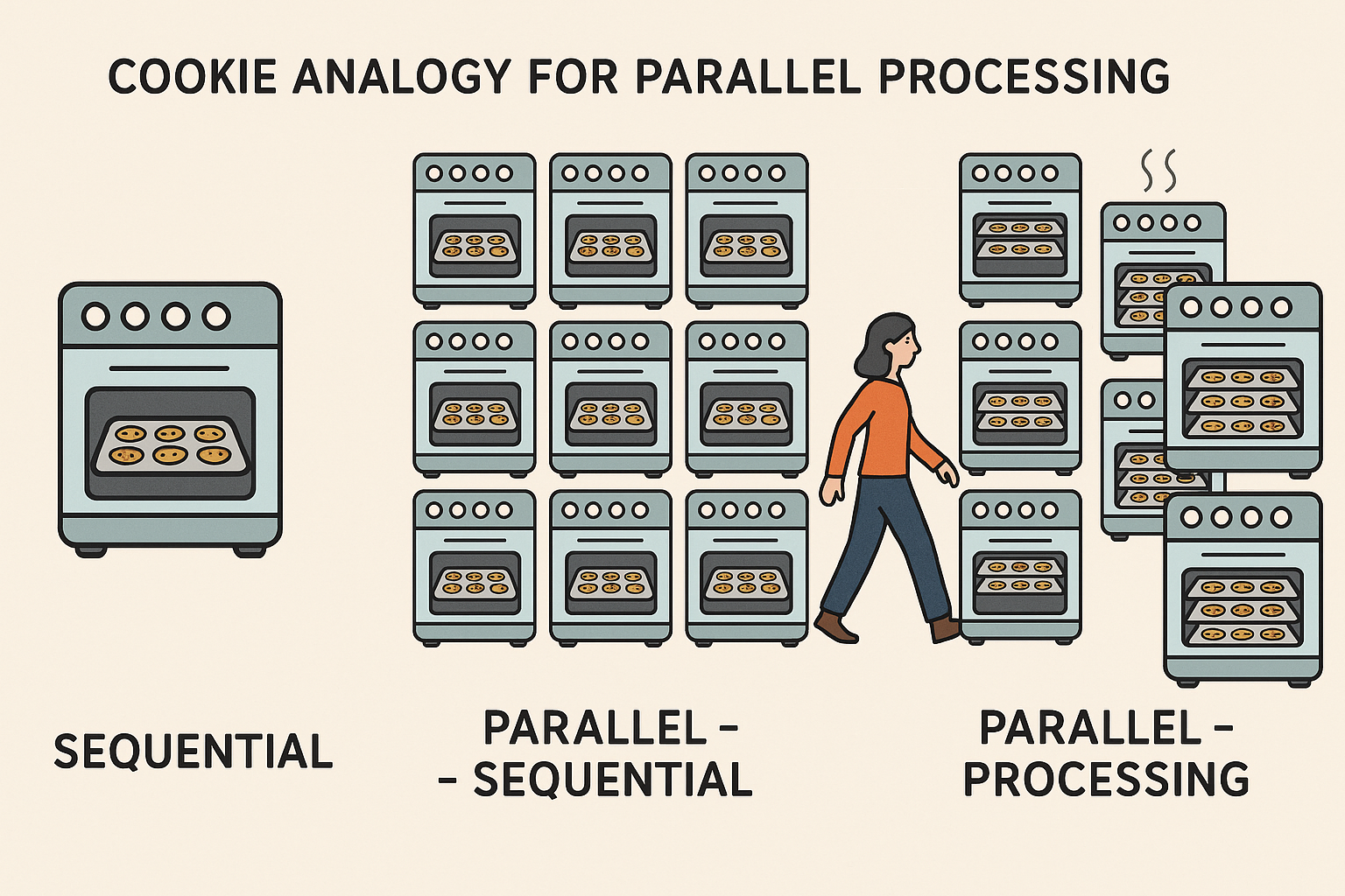
When activating parallel processing tasks are divided into equally sized chunks and directed to multiple CPU cores. Imagine you are baking cookies, in a sequential mode you would use one tray in one oven at a time. Moving to parallel-sequential, here you would use 10 ovens for baking your cookies but only with one tray in each oven. However, in parallel-processing you would use 10 ovens and and multiple trays in each oven at the same time. Thus, when working with so many ovens and trays maybe cookies will burn and you would have to walk between all the different ovens, that is what is called overhead. Overhead is the extra time, resources and effort needed to manage a task, apart from the task itself. In parallel-processing managing multiple threads, sending data to each chunk, retrieve results and synchronizing requires time and memory i.e. overhead. It is the cost of making things faster (R Core Team 2025).
The time to run e.g. poly_link() function depends on the number of grid cells i.e. sample size and the time of interest (TOI). The nested loop first iterates through each sampled grid (e.g. different amount of polygons) and then through different TOI. The tictoc package can record the time for this process. For smaller chunks parallel processing creates more overhead and is less efficient. Larger chunks reduce the overhead and perform generally better. For the gxc-package parallel-processing shows the best performance especially for larger sample sizes.
Increasing processing speed
What can you do when your operations are running slow? The performance of gxc operations is closely tied to the characteristics of your input data and the indicators you select. Working with large datasets—especially those typical in Earth Observation (EO), such as baseline temperature downloads or high sample sizes—naturally increases processing time. This also applies to wide spatial extents and longer focal or time-of-interest periods.
In general, both the quality and quantity of your data influence how efficiently the package performs. Be mindful of your system’s cache and critically assess which input data are essential for your research goals. Striking the right balance between data volume, processing time, and result quality is key to optimizing performance. Later, we will discuss the advantages of parallel processing to enhance the packages performance.
You can use the parallel-package in base R (function like lapply(), sapply() or apply()) for parallel computing. In the case they run slow you can apply interfaces to other languages like complied code in Rcpp. A code profiler like the profvis-package can help you find the bottleneck of your code i.e. where the slow code lies. Moreover, your code structure and order affect performance and speed. So start:
Sorting and ordering with algorithms like
c(“shell”, “quick”, “radix”)Converting data frames to (sparse) matrices
Using specialized row and column functions e.g.
apply()-functions from thematrixStats-packageDefining a memory directory
Avoiding copies
Vectorizing your code (works faster than loops)
Choosing the right data type (integers and factors work faster than characters),
Using bytecode compilation
Caching results
Employing
data.tableordplyr-functions
futureverse
The future-package is an API for sequential and parallel-processing. The package implements sequential, multicore, multisession and cluster features. Expressions can be evaluated on the local machine, in a parallel set of local machines or distributed on a mix of local and remote machines.
“Future is an abstraction for a value that may be available at some point in the future.” (Bengtsson 2024)
Futures can be created implicitly or explicitly, they can be resolved or unresolved and there are different ways of resolving a future. The way of resolution can be defined by choosing a fitting backend/ package e.g. sequential resolves futures sequentially and in the current R process whereas multisessionresolves futures parallely via a background R session on the current machine. The backend needs to be specified by the user to optimize functionality though there are some defaults for all backends:
- evaluation on local environment (unless defined otherwise),
- global variables are identified automatically,
- future expressions are only evaluated once.
Synchronous futures
Synchronous futures are resolved one after another. The main process is blocked until the resolution is completed. Sequential futures are the default backend in the future-package. They operate similar to regular R evaluation. The future is resolved in the local environment in the moment it is created.
Asynchronous futures
Asynchronous futures are resolved in the background and do not cause blocking of other tasks/ operations. You can carry on like that until you request a result of a still unresolved future or try to start another future while all background workers are busy, then the process will be blocked. The cookie-analogy: You can start prepping the next batch of cookies while the first one bakes but when the ovens are full you will need to wait to bake it or taste the ones that are still in the oven. Multisession futures are evaluated in background R sessions launched by the package running on the same machine as the calling process. Further processes/ tasks are locked when all session are busy. You can define a number of background sessions with the availableCores() function otherwise all available cores will be used. Multicore futures works with forking i.e. splits worker from the main session, both working on the same task. This can reduce overhead due to shared memory thus when changes are made a copy for the worker on the main session is needed and generally multicore futures tend to be instable. Cluster Futures creates a cluster of workers i.e. a team that works on the same task at the same time. Cluster futures can be local or remote, clusters that are not used anymore will be shut down automatically.
“Nested topology”
Nested futures can internally create another future, these futures are evaluated sequentially so that overload is avoided. Also the inner futures are set to sequential so one keeps control of further workers. With plan()you can change the mode of process to multisession, multicore and so on. For nested parallelism plans you can set multilevel plans:
plan(list(multisession, multisession))When working with nested futures it is important to keep management of the workers. Nested futures can easily cause memory overload, delays and failed futures caused by a lack of available R sessions.
…
Why is information on performance important?
Testing, documentation, and performance evaluation are critical throughout the development of an R package. These practices ensure reliability, maintainability, user trust, and a positive user experience. A well-designed package should produce correct and transparent results, function consistently across systems and R versions, and offer performance suitable for real-world applications. Clear documentation, intuitive interfaces, and informative error messages enhance usability and minimize the risk of misuse (Wickham & Bryan 2023).
How are we assessing performance?
CRAN’s standards for package submissions check for performance and correctness. CRAN has established a set of policies regarding quality, copyright, effectiveness and performance (R Core Team).
Literature
R Core Team. (n.d.). CRAN repository policy. The Comprehensive R Archive Network (CRAN). https://cran.r-project.org/web/packages/policies.html
Wickham, H., & Bryan, J. (2023). 18 Other markdown files. In R Packages (2nd ed.). https://r-pkgs.org/other-markdown.html